A Western Washington Tornado

Well, with a new year I decided it was time for me to resume my blogging activities.  So, I'll try to have regular updates on a weekly/biweekly basis at least as new weather topics come to me.

On Sunday afternoon, January 18th, most people in the Puget Sound area were glued to the television to watch the Seahawks game.  Passing outside their windows was a series of strong showers following a cold front, not at all unusual for the mid winter here.  Just before 2:30 PM PST the National Weather Service started getting reports of a tornado near Gig Harbor, Washington.  Here is the 0.5 degree base reflectivity radar image from the time.  Several strong, but compact cells across the southern Puget Sound lowlands.  Nothing that screams "tornado"...

It wasn't even the most intense cell that ended up attracting the attention here.  That cell produced hail later on, though at the sub-severe level.  No, it was the little blip to the west that produced an EF-1 tornado on the southeastern Kitsap Peninsula.  Here's the National Weather Service Seattle WFO storm survey results:

We joke about some of the storm damage markers we get from tornadoes in western Washington.  "Skylight cover sucked off".  "Kayaks moved around."  Though it's too bad that all tornadoes can't be this tame.

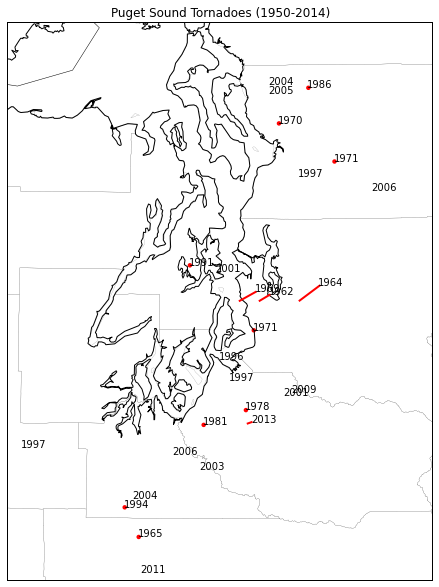
This has gotten me thinking about tornadoes in western Washington.  We get a few episodes with waterspouts every year, but tornadoes themselves are not very common.  I went back to the Storm Prediction Center's Severe Weather Database that I used in a previous blog post.  This includes a record of all known tornadoes since 1950.  It turns out in Washington state west of the Cascade Crest there have been 46 tornadoes since 1950 (47 after Sunday's event).  Here's a map of the tornadoes in the immediate Puget Sound area, labeled by year:

Those without red dots had path lengths too short to show up.  Given the short paths, relatively weak strength and the large amount of rural/undeveloped area in this region, there are probably more that escaped detection.  But there are actually more than I thought there would have been.

Another unusual feature of these tornadoes in the seasonal climatology.  Here is a histogram of the number of tornadoes per month (sample size of 46).

There's an odd sort of bimodal distribution here, with a rapid increase in number from March through June, then NONE in July, followed by a secondary ramp up in the fall through November before none in December and February.  Granted, this is a small sample size, but it's interesting that the tornado probability seems to crash so rapidly at the end of Spring and Fall.

Severe, tornadic storms and upper-level forcing

Just thought I'd quickly share this one screen capture I grabbed yesterday during the unusual November tornado outbreak over the Midwest.  I find myself more and more often using Weather Underground's "Wundermap" tool to overlay weather model output on current observations, satellite and radar to try and both see how well the model is doing and make connections between model features and what's actually happening.  Here we see the composite radar image over the continental US overlaid on top of the ECMWF 300mb forecast for around 1 PM CST on Sunday.  The 300mb wind speeds are shown in color with the 300mb height lines shown as the white contour lines.

You can really see how these lines of convection in the radar imagery formed along the exit region of the upper-level jet streak.  This is a favorable location for divergence aloft, particularly when the jet streak has cyclonic curvature as it does here.  Furthermore, the surface cold front associated with this storm was actually back over central Illinois at this time.  It was upper-level support out ahead of the cold front---this strong jet streak coming around the base of the trough---that provided a lot of the forcing to get this convection going.  Of course, once these storms organize into line segments they can be self-reinforcing in generating enough lift to keep themselves going.  But once again, this emphasizes how understanding what's going on in the upper-levels (something our models forecast fairly well) can be both useful and important for understanding when and where convection is going to develop (something our models don't do nearly as well).

The frequency of strong tornadoes

Given the recent EF5 Moore tornado, the 2011 Joplin EF5, the 2011 Tuscaloosa EF4 and other strong tornadoes in the last few years, a lot of people have been commenting on whether or not we're seeing more violent tornadoes now than in the past.  A few have even tried ascribing recent violent weather to climate change.  I find this particularly amusing, particularly consider that these last 12 months have been the least active 12 months of tornado activity on record.  But what do the trends say--are we seeing more strong or violent tornadoes more frequently?

A lot of people have looked at this particular question, including some excellent blog posts like those from  Jeff Masters.  A timely article in the Bulletin of the American Meteorological Society by Kunkel et al. shows that the frequency of strong (EF1+) tornado reports is not increasing, though weaker (EF0) tornado reports have increased.

Number of tornadoes per year (From Kunkel et al. 2013)

However, they note that these observations are complicated by many different factors, most notably the expansion of population areas over time and the increased prevalence of automated observations.  Because of these factors they looked at changes in the frequency of weather conditions that favor strong tornadoes instead.

Let's dive into these counts a little deeper to illustrate why it's difficult to pull any trend out of these numbers. I pulled a Patrick Marsh and grabbed the tornado count data from the SPC website and made the same sort of plot as the Kunkel et al. plot above, but for all of the different F/EF ratings.  On the left we see the counts of the total tornadoes reported each year in each strength category and on the right we see these counts as a fraction of the annual total.

In terms of raw numbers of tornadoes reported, the number definitely has been increasing over the last 53 years. However, we can see that it really has been those F/EF0 reports that have been driving the increasing trend in tornado reports.  If we look at the percentage plot on the right, we only see an increasing trend for F/EF0 reports--there is virtually no trend in the fraction of F/EF 1, 4 or 5 with slight downward trends (in terms of total fraction in F/EF2 and F/EF3 reports.  This is an interesting breakdown, particularly in the divergence between the reports of F/EF1 and F/EF 2 tornadoes.  This seems to be the breaking point--the total number of F/EF 1 and F/EF 0 tornadoes reported has been increasing while other levels haven't shown a whole lot of change.

A lot of this increase in reporting weaker tornadoes has to do with population growth as we urbanize more areas and a general increase in public awareness.  If you have strong tornadoes (here, F/EF 2 or greater), they're typically more likely to be reported; the damage is a lot more obvious and more easily attributable to tornadoes.  As we increasingly build up our urban areas and become more interconnected, we've become more sensitive to even small disruptions in our infrastructure and as such even damage caused by weak tornadoes gets reported.

I'm also curious as to the sudden jump in the number of  F/EF0 tornadoes that began in the late 1980s and has continued through this day.  I was wondering if this coincided with the roll-out of Doppler radars nationwide that took place in the late 80s and early 90s.  It turns out that a 2005 study by Simmons and Sutter looked at the impact of our Doppler radars on tornado warnings.  They broke down (on a forecast office-by-forecast office basis) the number of tornado reports by F-scale before and after the WSR-88D implementation:

From Simmons and Sutter (2005)

We can use these numbers to plot out the percent change in total number of tornado reports of each F scale category before and after Doppler radar implementation.

The percentage of reports of F0 tornadoes increased by about 11 percent--the only category where this happened.  I really think that the Doppler radar implementation has had a significant role in increasing the number of weak tornadoes reported, as this has allowed meteorologists to see small-scale spinups that might otherwise have been lost in larger thunderstorm wind damage.  This increased detection of weaker tornadoes helps focus storm survey efforts and attributes more damage reports to weak tornadoes than we may have suspected in the past.

So, after that brief look, it's true that the number of tornadoes reported has been increasing over time, but that doesn't necessarily mean that the total number of tornadoes has been increasing over time--we're just getting better and detecting weaker tornadoes and our population is more sensitive to the effects of weaker tornadoes.  In focusing on stronger tornadoes, there's not enough evidence to suggest that the number of reports are increasing.  In fact, as a fraction of total reports, the amount has remained somewhat steady if not decreasing slightly as weaker tornado reports have become far more common.

Using Doppler, dual-pol radar to interrogate storms

Last night there were some pretty impressive-looking storms that moved across northern Oklahoma, dropping a few tornadoes along the way.  I pulled a few screenshots of radar images from these storms to look at a lot of the helpful and hazardous things that our radar system gives us.

First, one of the primary advantages of having a Doppler radar--that is, a radar that uses the Doppler effect to measure wind velocity--is that it lets us more accurately see areas of rotation within thunderstorms.  Before we had Doppler radars (and we just had regular radars), all we had was reflectivity to look at.  Sometimes we got lucky and tornadic storms would produce a well-defined "hook echo" that let us know where a tornado was likely to be.  Here's an image (borrowed from Cliff Mass's blog, where he borrowed it from someone else) of an old-style, 1960s era radar image:

This works out great if you have a storm that has a well-defined hook echo structure.  But we don't always see clear hook echoes in tornadic storms.  Take a reflectivity image from last night, for example.

There are tornado warnings out for these storms and storm spotters reported a tornado on the ground with at least one of them at this time.  But where is the tornado?  There are a few candidate locations that look a little like hook echoes, but nothing too clear.

This is where being able to see Doppler wind velocities is really helpful.  Here's the base velocity image from this time:

I've circled the areas where there are nice velocity couplets that clearly show locations of strong circulation where there could potentially be tornadoes.  If you want to know a bit more about how to look for rotation in these radar velocity images, I wrote a blog post some time back about it that can be found here.

So getting Doppler radars was a huge boon to our ability to forecast and warn for tornadoes.  In fact, a lot of research suggests that adding Doppler capabilities to our radars is the single most important advance we made to increase our warning lead times and probability of detection of tornadoes.

But now we've added even more capabilities to our radars--this whole dual-polarization business.  What can dual-pol show us about these thunderstorms?

If you go through the training material for dual-pol, there are a lot of nice, relatively clean examples that are given that show you how to differentiate between things like rain, hail and even tornadic debris using dual-pol products.  However, in my experience, real-world interpretation of these products is often not nearly so clear-cut.  There are some things that dual-pol nails every time and other things that it doesn't.  Let's start looking at the dual-pol images from the time I showed above.

We'll start with differential reflectivity.  In dual-pol parlance, this is simply the difference between the strength of the horizontally-oriented radar return and the vertically-oriented radar return (eventually I'll write a more detailed blog post about all of this).  This means that the bigger and fatter objects (like, big raindrops which tend to flatten out as they fall) will have higher ZDR (differential reflectivity) values.  Nearly spherical objects or objects that are tumbling as they fall (like hail) will tend to have much lower, near zero ZDR values.  If you have a lot of different objects in an area (like, for instance, if there is tornadic debris being thrown around) we'd expect to see very noisy ZDR values.  Here's my annotations on the ZDR radar image for the time above:

There's a lot going on in that image.  Let's start with my top comment.  If we compare this to the reflectivity image above, you'll notice that in an area where there's a lot of high reflectivity to the north of the potential tornado, we see low, zero, or nonexistent ZDR.  This can happen if the radar beam is traveling through so much material (so much rain or hail) that too much of the beam gets absorbed to make reasonable inferences about what we're actually getting back from the radar beam.  There's just too little left to work with.  This is a phenomenon called attenuation--the absorption of the radar beam by some material that decreases the radar beam's power and resulting sensitivity.  I'll get back to that again later.  For now, it's somewhat disappointing that this northern part of the storm seems to be missing a lot of signal.

Just south of that, closer to the core of the storm, we have a patch of higher ZDR--on the order of 6-7 dB.  We know that higher ZDR values ten to correspond to big, flat objects like big raindrops. So we could probably infer that there was a very heavy downpour going on in the middle of the storm.

But what about the area right near the potential tornado?  The ZDR values are somewhat weaker there, though still slightly positive.  We know that near-zero ZDR values are typical of hail, so maybe there is hail there?  They also look a little noisy, and the base velocity image suggests there could be a tornado there.  Perhaps this is a debris signature?  It's really difficult to tell.

Let's try looking at another dual-pol image for help--the correlation coefficient.  Correlation coefficient basically tells us whether or not everything the radar beam is bouncing off of in that area of space is the same thing or not.  If we have high correlation coefficient, we're probably looking at all rain or all hail.  Lower correlation coefficients mean more of a mix of different precipitation types.  Really low correlation coefficients mean that what the radar beam is bouncing off of is probably not normal precipitation and is instead something like debris, bugs, dust...

Here's the correlation coefficient image from the same time.

Let's start with that area to the north of the core of the storm again, where we saw the low to nonexistent ZDR before.  We see here that that area is full of very noisy, lower correlation coefficients. This could either mean that we're seeing a lot of different sized and shaped objects floating around in that area, but another way to get low, noisy correlation coefficient is for there to be a very weak radar signal.  This is consistent with my early statement that the radar beam is probably somewhat being attenuated in that area.

Looking back down toward the area with the potential tornado in it, we see that the correlation coefficient is still quite high in that area.  This isn't very consistent with debris, as tornadic debris is all different shapes and sizes and should have a lower correlation coefficient.  So, high reflectivity with lower ZDR and high correlation coefficient makes me lean more toward hail being seen in this area.  But, it's very difficult to tell.  Even though we get so much more information from these dual-pol products, it still can be very difficult to interpret.

Let's look at a slightly later time when the storms had merged more together.  Our old friend reflectivity can show us a lot about the storm structure:

One of the striking features of this reflectivity image is the clear outflow boundary seen on reflectivity.  This is a narrow band of slightly higher returns that's making an arc shape out in front of the main storms.  An outflow boundary is the leading edge of the cool, downdraft air that accompanied the rain falling out of the thunderstorms.  As this cool air falls to the ground with the rain, it spreads out and races along the ground out away from the storm.  Those higher returns along the leading edge of the boundary are not actually caused by rain--they're caused by dust, dirt, insects and birds that are caught along the leading edge of the advancing air.  Want proof of this?  We only have to turn to the correlation coefficient image from the same time:

Remember that hydrometeors like rain and hail tend to be rather highly correlated--they're the same everywhere.  Even in mixed precipitation the correlation only drops a small amount.  But other things that are not so evenly shaped--things like dust, birds, insects--those show up as very low correlations.  You can see int he correlation coefficient image above that the outflow boundary is completely missing--the correlations of those returns are so low that they're actually off the color chart.  In fact, a lot of the clutter off to the west of the storms also basically disappears in correlation coefficient.  This highlights one of the best uses of correlation coefficient--to differentiate between what's actually precipitation and what's not.

Here's a look at the velocity image from this time.  Note the strong velocity couplets where there are potential tornadoes.  I've drawn in arrow to help show where the radar says the air is moving--remember green is toward the radar and red is away from the radar.  You can also see how the air behind the outflow boundary is moving to the south, out away from the storms.  There's also strong convergence right along the outflow boundary.

One final thing to look at here.  Sometimes when a radar gets hit with a particularly heavy downpour, the dome around the radar gets coated with a thin layer of water.  As the radar beam tries to pass through the radar dome, some of it gets absorbed by that layer of water, creating more attenuation.  Since the radar beam suddenly loses power as soon as it crosses through the layer of rain, it causes the beam's sensitivity to drop--we have less power going out, so there's even less power that can be reflected back.  This can make radar echoes suddenly appear weaker as a heavy downpour moves over the radar.  This happened last night.  Here's a reflectivity image from right before a downpour hit the radar:

Now watch what happens to the radar returns in the circled area in the next radar scan when there is a downpour right over the radar:

The strength of the return suddenly drops off!  This happens actually quite frequently, and we often call this the "wet radome effect".  Something to watch for if you suddenly see the radar echoes all weaken dramatically.

Outbreak

Nothing technical here tonight--just awe at how terrible the fury of nature can be.

Currently, the majority of the eastern US is under a tornado watch:

Fig 1 -- SPC tornado watches (red) and severe thunderstorm watches (blue) as of 0041Z, April 27, 2011.

With dozens and dozens of tornado reports so far.  Mississippi and Alabama have been particularly hit hard this afternoon--and storms are still continuing to move east.

Fig 2 -- SPC tornado, wind, and hail reports for April 27, 2011 as of 0041Z, April 28, 2011.

So to sum up the setup, here's the 00Z sounding from Birmingham, Alabama this evening:

Fig 3 -- Birmingham, AL, sounding from 00Z, April 28, 2011.

That's a practically uncapped environment with a surface-based CAPE calculate at 3458 J/kg--an enormous amount of convective potential energy from the surface layer.  The entire lower half of the sounding is potentially unstable--any significant lift is going to fire off storms.  And when those updrafts go up, what kind of wind shear are they running into?  Winds go from southerly at 15 knots at the surface immediately to 65 knots out of the southwest at 850mb.  This results in a 0-1km storm-relative helicity of 470 m^2/s^2.  That's an incredible amount of low-level wind shear, meaning a high potential for rotation in storms.  This is an environment with strong tornadic potential.

Everything just seems to be coming together for this event.  A deep, neutrally-titled trough in the 500-250mb layer aloft over the Mississippi Valley and a strong jet stream around its base are providing divergence aloft over much of the eastern US.  With surface dewpoints in the mid 60s or greater all the way from Tennessee up through Maryland, juicy air with lots of energy has nowhere to go but up.  Violently.

If you live anywhere where there's a tornado watch, please be extra vigilant.  We've already seen strong tornadoes move through places like Tuscaloosa, Birmingham, and even near Washington, DC.  To quote the SPC, this is a particularly dangerous situation.  Stay safe.

How to recognize rotation on Doppler radar

One of the most frequent questions I am asked by people is how we can see tornadoes on our Doppler radar.  Given that the shortwave that has trekked across the southern US the last few days has produced (and is still producing...) dozens of tornadoes, I collected a few images from radars to try and show the different signatures associated with tornadoes.  I believe that the more people know about looking for threatening weather, even in this sophisticated way, the safer we can be.  Nevertheless, personal diagnosis of radar images is no substitute for warnings from the experts at the National Weather Service.  Always pay attention to the warnings and advisories issued by the Weather Service--they're there to protect you.

Let's start with some basics.  The basic structure of a thunderstorm consists of two parts--warm, moist air rising in an updraft, and cool, rain-laden air sinking in a downdraft.

The kinds of thunderstorms that most often produce long-lived or strong tornadoes are called "supercells".  At the heart of a supercell storm is a rotating column of air called the mesocyclone.  Just because this rotating column of air is present doesn't mean that the storm is producing or will produce a tornado--all supercells have a rotating mesocyclone, but only some produce a tornado. The presence of rotation in the middle of a storm will somewhat twist and turn how the updraft and downdraft actually look.  Let's switch to an idealized block diagram looking down from the top of a storm.  The warmer, moister air is usually to the south or southeast of the storm, so that's where the storm starts drawing in its moisture.  Because there is a rotating core in supercells, it can draw in warm moist air somewhat laterally instead of just vertically.  This air that is drawn in is called the "inflow".

The inflow rises up as it enters the storm, forming the updraft.  As the warm, moist air rises, it cools off, and as the air cools off, water vapor condenses back out into liquid water and rain is formed.  Eventually, at the top of the cloud, there is rather cold, rain-filled (or hail and ice filled too) air that is no longer buoyant because it's so cold.  So, it starts sinking.  Now, for the storm to keep growing and maintain itself, the downdraft can't sink into the updraft--this would choke off the updraft and kill the storm.  But in an organized storm like a supercell, this doesn't happen.  The downdraft air takes one of two paths (usually).  A lot of the air gets pushed out in front of the updraft (to the east, typically) by the strong upper-level jets that we find at the top of the storm.  The same jet streaks that are providing the divergence aloft to support the updraft can also carry the cold, rain-filled air off ahead of the storm and away from the updraft.  Thus, we'd expect to see a lot of radar returns out ahead of the mesocyclone area, since radar beams reflect off of raindrops.  This large area of precipitation and sinking air out in front of the mesocyclone is called the "front flank downdraft".

However, because the center of the storm is rotating, some of the downdraft air can get wrapped around the back side of the storm as well.  Thus, in most supercells, we see an intense, though narrow band of rain wrapped around on the back side of the mesocyclone.  This part of the downdraft is usually called the "rear flank downdraft".  Here's a block diagram of the two paths I just metioned:

So what would our resulting radar reflectivity image look like for this kind of situation.  We expect to see lots of returns out ahead of the storm because that's where most of the rain-filled downdraft air is going.  There would also probably be a weaker area of returns (or no returns) where the inflow region happened to be, since that warm, buoyant and rising and rain is probably not falling through that area.  Then we also expect a narrow band of radar reflectivity returns behind the mesocyclone corresponding to that portion of the downdraft that gets wrapped around by the rotating air.  The light green outline here shows generally what we'd expect to see on radar:

Basically we expect to see radar reflectivity returns everywhere that the downdraft is dominant.  Does this structure start to look familiar?  This pattern of reflectivity return is the iconic signature of a supercell thunderstorm.  Notice how since the rear flank downdraft--the downdraft air getting wrapped around the mesocyclone--is forced out into the inflow air, and there is a protruding area of reflectivity return on the southern side of the storm.  This defines what is commonly called the "hook echo" that you so often hear about on TV. Hook echoes are a sign of a strong rear flank downdraft coupled with a strong inflow region.  This is only really feasible if you have very strong rotation in the storm.  Notice how there is no real reflectivity return in the inflow region.  Because air is rising in this region, no rain is falling there and we get no radar return.  However, this seems to "notch out" the otherwise round reflectivity signature of the storm.  This area of no return cutting into the storm is referred to as the "inflow notch".  It helps define the hook echo and shows you the area where the storm is bringing in its warm, moist air.  A deep inflow notch often means strong inflow and updrafts and correspondingly a strong storm.

So what does this look like on an actual radar reflectivity image?  Here's a picture of a radar reflectivity image from a supercell thunderstorm from this afternoon in North Carolina that was producing a tornado at the time:

Radar 0.5 degree Base Reflectivity image from KRAX, 2040Z, April 16, 2011. 

I've overlaid labels of several of the features we talked about.  You can see all that enhanced return to the north and east of the center of the storm--that's all rain and hail falling in the front-flank downdraft region.  That sharp cut into the reflectivity on the eastern side is the inflow notch--this is the area where the storm is drawing in its warm, moist air.  Rising motion dominates here, and as such no rain is falling (and we see no reflectivity returns).  However, there is a clear, hook-shaped appendage hanging down from the storm--a classic hook echo.  This is that other part of the downdraft air (the rear flank downdraft) that is wrapped around the mesocyclone as it descends, bringing rain (and, consequently, radar returns) with it.  Some of that enhanced return in the big ball at the end of the hook might actually be the radar reflecting off of debris being kicked up by a tornado on the ground.  The hook echo and the inflow notch wrap around the area of strongest rotation--the mesocyclone.  If the mesocyclone becomes very tightly wrapped at low-levels, it can form a tornado.

So that's all and good for reflectivity images--we can recognize these kinds of structures that show us what rotation is doing to the environment.  But what about seeing rotation itself--looking at the wind velocities?  Our Doppler radars can do this, and that's a big reason the Doppler capability was added to the radars.  They do have some limitations, though.  But first...let's get back to concepts.

We have an area of strong rotation in the mesocyclone. Winds there are probably much faster than they are elsewhere, and they also change speed and direction over a very small spatial area.  Our Doppler radars can measure wind speeds, but only in two directions--air moving toward the radar and air moving away from the radar.  The radar measures wind speed by looking at phase differences caused by moving targets along the radar beam.  However, things moving across the radar beam perpendicular to it do not cause phase shifts along the beam.  So, we can actually only measure wind in two directions--towards and away.  Turns out that's all we really need.

Let's go back to the mesocyclone diagram and insert a theoretical radar location.  Since the radar measures winds moving toward and away from it, the radar's location is going to dictate what the return looks like.  In the image below I've randomly added a radar located to the southeast of the storm.

As the radar looks toward the storm, its beam follows a path similar to the dotted line.  You can see that to the right of the dotted line, winds in the mesocyclone (which is rotating counter-clockwise here as most mesocyclones do...but that's a topic for another blog...) are generally moving away from the radar.  But, to the left of the dotted line, winds are generally moving toward the radar.  We can assume that if there's a compact space where winds suddenly shift from moving away from the radar to moving toward the radar, there's probably something rotating there.  Unfortunately, we just can't tell what's going on when winds are blowing perpendicular to the radar beam (unless you use another radar located at another location, for instance).  But, in general, anything rotating should have one side strongly blowing away from the radar and the other side strongly blowing toward the radar.

What will this look like on a radar velocity image?  Usually, warm colors like reds and oranges are used for winds blowing away from the radar.  Cool colors like greens and blues are used for winds blowing toward the radar.  If we assume that the rotation is very concentrated in the mesocyclone, we'd then expect the radar velocity return to look something like this:

We'd expect a small area of bright reds (or oranges, or other warm colors) to be located right next to a small area of bright greens (or some other cool color) with a line parallel to the radar beam running in between them.  This is important--the red and green enhancements must be on either side of a line drawn radially outward from the center of the radar.  If they are not, it implies other things (like convergence or divergence--which are also important, but not rotation...).  The reds once again indicate air moving away from the radar and the greens indicate air moving toward the area.  If they are right next to each other, that implies that the winds are changing very rapidly across a small-distance--and that there's probably strong rotation.

What does this look like in real life?  Here's the base velocity image corresponding to the radar reflectivity image of the storm in North Carolina that I showed above.

Radar 0.5 degree Base Velocity image from KRAX, 2040Z, April 16, 2011.

Note that in the radar image above, the radar location is actually off to the upper left side of the image.  I've drawn a black dotted line along what is approximately the radar beam path.  Notice how there's a very localized area of bright green colors right next to an area of bright red colors exactly where we guessed the mesocyclone to be from the reflectivity image.  If you follow the arrows I drew showing the approximate rotation of the mesocyclone, you'll see that the bright green side corresponds to air moving toward the radar and the bright red side corresponds to air moving away from the radar.  So...here we have a rotation signature right where we expected it to be--in the mesocyclone region.  This close pairing of bright red and green colors on the radar is known as a "velocity couplet". It's a hallmark of rotation.

So those are the basics.  Now let's look at a couple more examples, just for practice.  Here's a reflectivity image of the powerful supercell and tornado that did lots of damage right as it moved over downtown Raleigh, North Carolina.

Radar 0.5 degree Base Reflectivity image from KRAX, 1940Z, April 16, 2011.

Once again, off the north and the east of the storm is the front flank downdraft--where most of the downdraft air, hail and rain is falling.  We see an inflow notch cutting in and a strong hook echo wrapping around the bottom side of the storm.  Right in between we would expect to see the mesocyclone and tornado.  You can really visualize in these reflectivity images how the mesocyclone is wrapping things up around it, forming that hook echo. How does this look on the velocity image?

Radar 0.5 degree Base Velocity image from KRAX, 1940Z, April 16, 2011.

The couplet is not as strong, but there's lots of air inbound to the radar on the southern side of the mesocyclone.  You can actually see where the radar is located in this image--in the middle of that black circle on the lower right side.  Once again, if you match up the arrows I've drawn showing the rotation to the colors, you can see that there's green on the side where the air is blowing toward the radar and red where the air is blowing away from the radar.  It matches up very well.

Of course, you'll notice on these velocity images that there are a lot of places where green and red velocity colors are right next to each other--and obviously they don't all mean rotation.  This is why I also discussed the reflectivity images--it's best to use the reflectivity images to know where to look for rotation before looking at the velocity images to verify your suspicions. If you just use the velocity images, you can sometimes get rather lost.

But, then again, sometimes the reflectivity images don't tell you everything and don't show the clear structures we saw in today's North Carolina storms.  For example, here's another tornadic supercell in Oklahoma two days ago in reflectivity:

Radar 0.5 degree Base Reflectivity image from KTLX, 202Z, April 15, 2011.

Not the clearest-cut structure here.  You might guess that that sharp cut of lower reflectivity values into the southern side of the storm could be an inflow notch.  But, then the hook to the west of that really doesn't look like a hook.  This is what's called an "HP supercell" for 'high precipitation".  When there's a whole lot of rain or hail, sometimes there is so much reflectivity return in different places that it can mask the signatures of rotation that would otherwise have been seen in the reflectivity.  But it's a strong enough storm that a look at velocity is warranted.  Here it is:

Radar 0.5 degree Base Velocity image from KTLX, 202Z, April 15, 2011..

Wow--that's some intense rotation right there.  I drew in the arrows again to show the area we're looking at.  The radar is located off to the northwest of this storm.  That's a very strong velocity couplet indeed.  But, the evidence of this rotation was somewhat hidden in the reflectivity image.  Also, the further you get from the radar, not only does your resolution decrease, but your radar beam is getting higher and higher above the ground.  This storm is rather far from the radar, and we're probably not looking at the "low-level" features of this storm.  Nevertheless, this storm is clearly rotating and with a strong velocity couplet like that, it's no wonder it was producing a tornado.

As I said before, often it can be somewhat difficult to really tell what is rotation and what's not by just looking at the velocity image alone  Often, as we saw above, the reflectivity image may not be very much help either.  In these cases, you just have to investigate and be persistent--check higher tilts of the radar to see if there's clearer signs of rotation aloft, look at a loop of images to see any suspicious signs in the recent past, and so on. However, the velocity couplets for strong storms will usually stand out.  Just as an exercise, here's a wider view of the reflectivity images of the storms in eastern Oklahoma on Thursday evening:

Radar 0.5 degree Base Reflectivity image from KSRX, 231Z, April 15, 2011.

A mess of several nasty storms.  Could that be a very fat hook echo on the southwest side of the furthest northeast cell?  Or what about the smaller appendage sticking out of that same cell just to the east of the fat hook?  And what about these other cells further to the southwest--they're definitely intense, but do they have rotation in them?

Here's the raw velocity image for that same time:

Radar 0.5 degree Base Velocity image from KSRX, 231Z, April 15, 2011.

There's a lot going on in that velocity image.  Can you spot areas that may be rotation?  On the image below I've circled some of the areas that I would want to look at more closely.  Some are pretty obvious...others are just suspicious enough to warrant a look:

Well, that's all I have for now.  I hope this has given you enough background to start spotting potentially rotating storms on radar.  Once again--just because a storm is rotating doesn't mean it's producing a tornado. And, even more importantly, just because you don't think you see any rotation on the radar but the Weather Service has a warning out does not mean you should ignore the warning. There are professional meteorologists whose job it is to analyze radar images and lots of other data to determine what is going on and who to warm.  Trust their judgment and take cover when there's a warning.

Thoughts on Severe Weather Sunday Night, Part 2

Now that I'm back again, to continue the discussion.  I already noted in part one how the upper-air pattern seemed somewhat chaotic in the forecast and that would also reflect on the surface pattern.  It's the surface and low-level variables that really have people worked up about this event.  Remember how we saw a strengthening pressure gradient due to pressure rises and falls across the middle part of the country?  That means increased southerly winds across the plains and the midwest.  With those winds comes strong advection of moisture and warm air northward.  Here's the NAM model forecast for dewpoint temperatures tomorrow evening:

Fig 1 -- NAM 36 hour forecast of dewpoint temperatures (colors) and winds (barbs) for 00Z, Monday (Sunday night), April 4, 2011.  From the HOOT website.

Note that the 60 degree dewpoint contour is all the way up to northern Illinois and eastern Iowa by Monday evening--that's very far north to be seeing dewpoints that high.  Particularly when the 70 degree dewpoints (the darker greens) are still confined to the Gulf of Mexico.  The southerly winds are very evident within that tongue of moist air moving north.  However, the wind pattern and the shape of that warm, moist sector are somewhat odd on the western side.  Note we have several westward "bumps" in the moisture coincident with strong wind shifts.  These are marking areas of perceived low pressure and surface boundaries.  I personally would interpret the above pattern like this in terms of surface features:

Fig 2-- Same as figure 1, but annotated with surface features by the author.

Each one of those "bumps" westward has somewhat of cyclonic flow around it and a quick check of the surface map (not shown) shows both areas to have relatively lower pressure than their surroundings.  So, both are labeled as "lows" on the map.  The leading edge of the moisture surging northward would be the warm front--that's pretty straightforward.  Strong north-westerlies behind the northern low look like flow behind a cold front, so I've drawn a cold front along that boundary.  Now, what's happening around the southern low is interesting.  Usually when we see a shift in the winds with north to northwesterly winds to the north and more westerly or southwesterly winds to the south, the wind shift to the south represents a dryline and the winds to the north show a cold front.  This wind shift also seems to extend westward behind the southern low.  I've labeled it with a dotted line above, indicating some kind of surface trough.  However, all I believe has happened here is that the cold front associated with the northern low is overtaking the dryline to the south.  Eventually those northwesterly winds behind the cold front will sweep in behind and there will be no more dryline.  The places where these boundaries intersect are known as "triple points", and you may see them mentioned in weather discussions.  That southern "low" would be considered a "triple point" since it's an area where three boundaries meet--the cold front, the dryline and the surface trough.  Areas near triple points in the moist region (so, to the east in the above map) are often favored areas for severe weather development.

So we see a complex suite of boundaries and low pressures in the forecast--reflective of the complex upper-air pattern we saw above.  The boundaries (and to an extent the upper-level winds) will provide the lifting mechanisms, and we can see in the dewpoint maps above that there is moisture available to work with.  We need two more things for severe storms--wind shear and instability.  With respect to wind shear, there is an awful lot of that.  The 850mb winds are forecast to be roaring out of the southwest on Sunday evening.

Fig 3 -- NAM 36 hour forecast of 850mb winds (colors) and geopotential height (contours) for 00Z, Monday (Sunday night), April 4, 2011.  From the HOOT website.

Those are 65 knot+ winds in the Ohio River Valley on Sunday evening.  Note that the wind swath seems a bit east of the fronts and the dryline, but there are still strong winds over the entire moist sector.  Even though the strongest winds may not be exactly over the region with the best forcing, there still are strong enough winds just off the surface for there to be plenty of low-level wind shear.

What about instability?  A good first glance at instability is to look at the surface-based convective available potential energy (CAPE).  The higher the CAPE, the more the instability.

Fig 4 -- GFS 36 hour forecast of surface-based CAPE for  00Z, Monday (Sunday night), April 4, 2011.  From the HOOT website.

Strong CAPE values are pooled near the dryline and cold front, but also extend out east (somewhat more weakly) into the warm sector.  But, just because there's CAPE doesn't mean that there will be storms.  That available convective energy is only "available"--any storms have to be able to tap into that.  With a strong lifting mechanism (like a cold front, for example...) it becomes very easy to tap into that energy because the lifting is being done by the advancing cold air behind the cold front.  As such, storms are much more certain to fire along the cold front up north as opposed to further south, even if the CAPE is higher to the south.

So what would be stopping storms from forming and becoming severe further south?  The answer is something called the "capping inversion".   Normally air cools with height--it's much colder further up in the atmosphere than it is near the surface.  In fact, the faster it cools off with height, the more unstable the air gets because warm air near the surface is more buoyant than the colder air above.  This promotes rising motion and the formation of thunderstorms.  In fact, in some ways, CAPE is a measure of how steeply the temperature cools with height (it includes other things like moisture content too...).  Generally, the faster the air cools with height, the more CAPE you have and the more unstable the air becomes.  The opposite happens in a "capping inversion".  This is a region of the atmosphere where the temperature actually warms with height.  This is bad for rising air because if it runs into air that is warmer than it is, the rising air is no longer more buoyant than the air around it and it will stop rising.  Capping inversions (or, "the cap" for short) are easy to see on vertical soundings.  Here's a NAM model forecast sounding for Norman, Oklahoma at 21Z on Sunday (Sunday afternoon):

Fig 5 -- NAM 33-hour forecast sounding for OUN valid 21Z, Sunday, April 3, 2011.  From the HOOT website.

The red line is the forecast temperature of the atmosphere as we go up in height, and temperatures decrease to the left in the image above.  See that strong kink in the temperature profile that I circled?  Generally the profile is slanting to the left--the temperatures are cooling with height.  But in that one layer the temperatures abruptly warm with height.  This is a capping inversion--it prevents air near the surface from easily rising above the cap.  If it could, it would have very good convective potential--the CAPE value listed on the above sounding is 1716 J/kg.  Generally anything above 500 J/kg is good for strong thunderstorms.  And the higher the number, the more energy available for convection.

So how would we get storms when there is a cap?  We'd have to break the cap somehow.  There are three main ways of doing this:

1. Cool the air above the cap
2. Warm the air below the cap
3. Have a cold front or some other strong lifting mechanism move in that can shove the surface air right through the cap regardless of its relative buoyancy.

Usually some combination of these does take place, though the second one becomes most dominant in the absence of a front moving through.  As the day wears on, the sun heats up the earth's surface more and more, causing the temperature at the surface to get warmer and warmer.  Also, turbulent mixing can bring warm air down from above the cap and cool air up from below the cap and sort of "even out" the temperature, making the temperature jump less abrupt.  This combination of things works to erode the cap--which is exactly what the NAM model forecasts to happen just three hours later at 00Z:

Fig 5 -- NAM 36-hour forecast sounding for OUN valid 00Z, Monday (Sunday evening), April 4, 2011.  From the HOOT website.

Just three hours later, the NAM no longer forecasts there to be a cap present!  The air near the surface is now warmer than all the air above it and parcels can rise much more easily now.  So according to this forecast, there definitely is potential for the cap to break down and for us to see some thunderstorms further south.  The OU/OWL WRF model shows a similar profile for 00Z Monday, lending further credence to this possibility:

Fig 5 -- OU/OWL WRF 48-hour forecast sounding for OUN valid 00Z, Monday (Sunday evening), April 4, 2011.  From the HOOT website.

The NAM soundings on the HOOT site stop at 00Z Monday, but the WRF model goes slightly further, and I want to use its soundings to show something.  All of these maps and soundings I've shown are at 00Z Monday, which is around 7 PM central time on Sunday night--right before sunset.  What happens if we go three hours later, to 3Z Monday (10 PM Sunday night)?  Here's the OU/OWL WRF forecast sounding for Norman at that time:

Fig 6 -- OU/OWL WRF 51-hour forecast sounding for OUN valid 03Z, Monday (Sunday evening), April 4, 2011.  From the HOOT website.

The cap has reappeared!  Why is this?  As soon as the sun goes down, the earth's surface really starts to cool off.  As it cools off, this in turn cools the air right above the surface.  However, the air in the low-levels of the atmosphere still retains its warmth from the day.  So, as the surface cools, so does the air right above it.  But above that, we still have very warm air.  Thus, another capping inversion sets up, where the air warms abruptly with height.  This prevents new storms from forming that draw on surface air for their energy, and also causes already-existing storms to elevate above the capping inversion.  When a storm elevates, it no longer draws in air from the near-surface layer of the atmosphere and instead must draw in air from above this layer.  This is in contrast to surface-based storms that draw in their warm, moist air from the surface layer of the atmosphere.  Since the capping inversion stops near-surface air from easily rising, any surface based storms that run into a capping inversion tend to lift above the inversion and start drawing in air from above that level.  They can still be severe, but usually elevated storms are not tornadic--a tornado has to extend to the ground and it can't do that (easily) if the storm is elevated.

Notice one other thing in the last two profiles I've shown--the low-level winds pick up in speed rather extraordinary between 7 PM and 10 PM (see the wind barbs between the surface and 700mb in the two soundings above).  This has to do with the nocturnal low-level wind maximum (sometimes associated with what is also called the low-level jet).  The details of why this happens are enough material for another whole blog post, so I'll just say that as the sun goes down (and as that capping inversion becomes re-established), the low-level winds tend to speed up rather suddenly.  This is good for severe storms as they need wind shear to maintaining rotating updrafts and produce hail, strong winds and sometimes tornadoes. However, this night time increase in winds occurs at the same time that the capping inversion shows up again, causing the storms to elevate.  This is why the time right around sunset is often critical if you are looking for tornadoes--you want the atmosphere to stay uncapped so you still have surface-based storms, but you also want the wind shear to increase.  Right around sunset sometimes the capping inversion hasn't quite started to creep in yet and sometimes the wind shear will really start kicking up and you'll see an increased risk of tornadoes around then.

However, with the increase in low-level winds comes an increased tendency for storms to form bow-echoes and have strong, straight-line winds associated with them, regardless of if they're elevated or surface-based.  We often see an afternoon full of isolated supercells and small storms quickly congeal together into big lines of storms after the sun goes down and the low-level winds kick up.

IN SUMMARY...

So, in summary of all this--models are coming into agreement that severe weather is possible across much of the central US.  We're virtually guaranteed to see storms further north from Iowa and Missouri into Illinois because the cold front should be moving through.  The cold front is such a strong enough forcing mechanism that regardless of if there is a cap, it can force enough lift to cause some strong thunderstorms.  Further south, the threat becomes more conditional in the afternoon as the models are forecasting a strong capping inversion at many places.  As we saw in the examples above, models are also showing that the cap may erode enough in the late afternoon and early evening that we could see some good storm development.  However, the cap is forecast to quickly become re-established as night falls, limiting the surface-based development and consequently the strong tornadic potential.  However, as winds pick up around sunset, the potential for lines of storms with strong winds increases.

We'll see how it all plays out tomorrow...

MD for the NW

It's not often at all that you see something like this out here in the Pacific Northwest:

Fig 1 -- Mesoscale Discussion 2128 from the Storm Prediction Center on Tuesday, Dec. 14, 2010.

A mesoscale discussion for this region?  Not only that, but a discussion about an isolated tornado threat for the Puget Sound lowlands down through the Willamette Valley? Very intriguing.  To see the full text of the mesoscale discussion, you can visit the SPC's page for it here.  They note that there probably won't be a watch because the threat is so limited.  However, there already has been a tornado report near Salem, OR.

Right now, there's just some scattered showers moving through the region.

Fig 2 -- 0.5 degree base reflectivity from KRTX radar at 2207Z, Dec. 14, 2010.

Some stronger convective elements are present, particularly in the storm east of Portland.  Some of the showers coming over the Coast Range to the west are also showing stronger cores.  Added orographic lift as the southwesterly winds aloft are forced to rise over the low mountains there seems to be helping to get some of the showers convecting.  A view looking south from the top of the Atmospheric Science building at the University of Washington in Seattle shows the rain to the south (but clear skies over Seattle!).

Fig 3 -- Southward view toward Mount Rainier (though you can't see it) from the roof of the UW Atmospheric Sciences building at 2:14 PM PST.  From the UW Northwest Observations website.

So why this isolated tornado threat for the area?  The big story is the wind shear.  Here's this morning's 12Z sounding out of Salem, OR.

Fig 4 -- 12Z sounding from Salem, OR, on Dec. 14, 2010.  From the SPC website.

Focusing on the winds, it's clear there's a lot of wind shear, both directional and speed-wise, going on in the lowest levels.  Winds go from southerly at 10 knots at the surface to westerly at 40 knots at 850mb.  That's a fairly large amount of wind shear, particularly for this region of the country.  In terms of instability, the lapse rate is conditionally unstable--it's steeper than a moist adiabat but not quite as steep as a dry adiabat.  The absence of any strong temperature inversion also helps make this a tempting sounding for instability.  There's clearly a lot of moisture and with just a little warming at the surface, a fair amount of CAPE could be generated.  There are many ways to get warming at the surface.  One way is through warm air advection--wouldn't you know that the surface to 850mb directional wind shear represents a veering of winds with height.  That's a sign of warm air advection going on.  You can also see in the sounding above that the SPC analysis tools have  picked up on this as well--the vertical bar chart labeled "Inferred Temperature Advection" shows red bars (indicating warm air advection) at low levels with blue bars (indicating cold air advection) in the mid levels.  Warming below and cooling above will tend to destabilize the lapse rate.

Of course another thing that will help warm the surface is clear areas where sunlight can get through.  Here's a look at the latest visible satellite image over Washington.

Fig 5 -- Visible satellite image over Washington state at 2215Z, Dec. 14, 2010.  From the College of DuPage website.

There's still a lot of stratus cloud cover over southwestern Washington and northern Oregon (you could even see that on the webcam image above).  But, Puget Sound is definitely clear.  There's also some isolated patches of clearing on the northern Oregon coast between areas of very convective-looking clouds.  This makes sense as strong convective updrafts usually have compensating downdrafts (or subsidence) that tend to clear the air around the storm.  This clearing lets sunlight get through and can further help to warm things up.

So, perhaps we'll see some more destabilization this afternoon--there's still a few hours of sunlight left.  And with that wind shear, we'll have to watch extra carefully to see if we spot any rotation.